Active learning is a subfield of artificial intelligence. It is curious to select the data which it learns during training.

Introduction

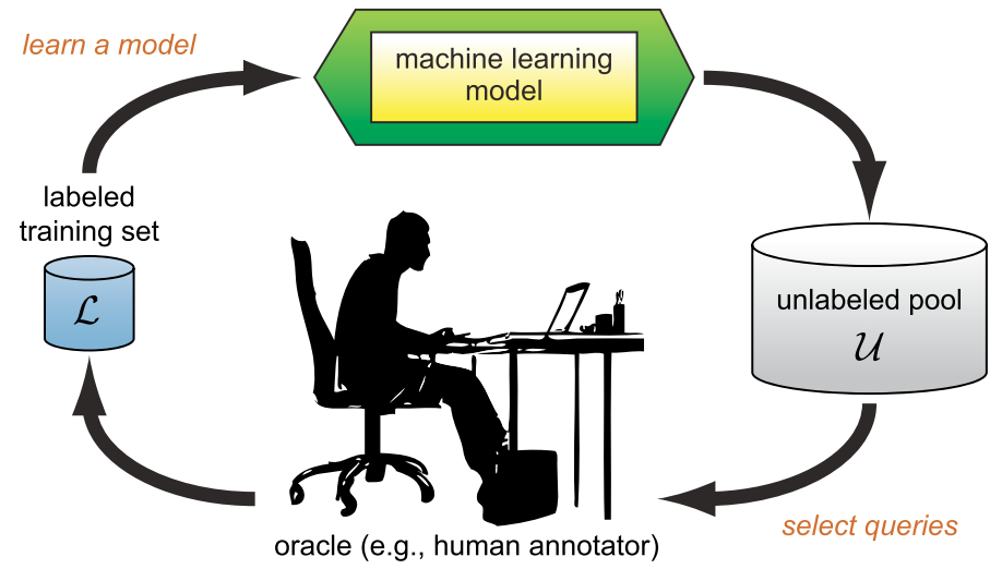
The key idea of active learning is that a machine learning algorithm can achieve greater accuracy with fewer training labels if it is allowed to choose the data from which it learns. Active learning may pose queries (asking queries), usually in the form of unlabelled data instances to be labelled by an oracle (e.g., a human annotator).

Active learning (AL), also called query learning, is a subfield of machine learning. It mainly focuses on the study of datasets. The key hypothesis is that if the learning algorithm is allowed to choose the data from which it learns (to be curious).

Active learning assumes that different samples in the same dataset have different values for the update of the current model, and tries to select the samples with the highest value to construct the training set.

For many other more sophisticated supervised learning tasks, labelled instances are very difficult, time-consuming. For instance, it may take ten times longer than the actual audio to annotate the word level. Locating entities and relations for knowledge graph or graphical neural network can take a half-hour or more for even simple newswire stories.

Scenarios

The pool-based active learning setting, in which queries are selected from a large pool of unlabelled instances $/mu$, using an uncertainty sampling query strategy, which selects the instance in the pool about which the model is least certain how to label.

There are three main settings, membership query synthesis, stream-based selective sampling, and pool-based sampling.

Code

Use different query strategies to get specific scores.

method(prob_dist.data[0])

And then, sorted the score from the largest to the smallest.

samples.sort(reverse=True, key=lambda x: x[4])

Finally, use step to sample data under specific score-order.

samples[:number:]

Full codes：

def get_samples(self, model, unlabeled_data, method, feature_method, number=5, limit=10000):
    """Get samples via the given uncertainty sampling method from unlabeled data 

    Keyword arguments:
        model -- current Machine Learning model for this task
        unlabeled_data -- data that does not yet have a label
        method -- method for uncertainty sampling (eg: least_confidence())
        feature_method -- the method for extracting features from your data
        number -- number of items to sample
        limit -- sample from only this many predictions for faster sampling (-1 = no limit)

    Returns the number most uncertain items according to least confidence sampling

    """

    samples = []

    if limit == -1 and len(unlabeled_data) > 10000 and self.verbose: # we're drawing from *a lot* of data this will take a while                                               
        print("Get predictions for a large amount of unlabeled data: this might take a while")
    else:
        # only apply the model to a limited number of items                                                                            
        shuffle(unlabeled_data)
        unlabeled_data = unlabeled_data[:limit]

    with torch.no_grad():
        v=0
        for item in unlabeled_data:
            text = item[1]
            
            feature_vector = feature_method(text)
            hidden, logits, log_probs = model(feature_vector, return_all_layers=True)  

            prob_dist = torch.exp(log_probs) # the probability distribution of our prediction
            
            score = method(prob_dist.data[0]) # get the specific type of uncertainty sampling
            
            item[3] = method.__name__ # the type of uncertainty sampling used 
            item[4] = score
            
            samples.append(item)
            
            
    samples.sort(reverse=True, key=lambda x: x[4])       
    return samples[:number:]

Query strategy frameworks

There are 8 common query strategies utilized in AL, uncertainty sampling, query-by-committee, expected model change, expected error reduction, variance reduction, and density-weighted methods. All AL scenarios involve evaluating the informativeness of unlabelled instances, which can either be generated de novo (start from the beginning) or sampled from a given distribution.

Simplex corners indicate where the one label has very high probability, with the opposite edge showing the probability range from the other two classes when the label has very low probability. Simplex centres represent a uniform posterior distribution. The most informative region for each strategy is shown in dark red, radiating from the centres.

Uncertainty Sampling

One of the most commonly used query framework is uncertainty sampling.

least confident

Query the instance whose prediction is the least confident:

$$x^*_{\text{LC}} = \underset{x}{\text{argmin}} 1 - P _\theta (\hat{y}|x)$$

where $\hat{y} = \text{argmax} _y P _\theta (y|x)$, or the class label with the highest posterior probability under the model $\theta$. One way to interpret this uncertainty measure is the expected 0/1-loss, i.e., the model’s belief that it will mislabel $x$.

Code

def least_confidence(self, prob_dist, sorted=False):
    """ 
    Returns the uncertainty score of an array using
    least confidence sampling in a 0-1 range where 1 is the most uncertain
    
    Assumes probability distribution is a pytorch tensor, like: 
        tensor([0.0321, 0.6439, 0.0871, 0.2369])
                
    Keyword arguments:
        prob_dist -- a pytorch tensor of real numbers between 0 and 1 that total to 1.0
        sorted -- if the probability distribution is pre-sorted from largest to smallest
    """
    if sorted:
        simple_least_conf = prob_dist.data[0] # most confident prediction
    else:
        simple_least_conf = torch.max(prob_dist) # most confident prediction
                
    num_labels = prob_dist.numel() # number of labels
        
    normalized_least_conf = (1 - simple_least_conf) * (num_labels / (num_labels -1))
    
    return normalized_least_conf.item()

margin sampling

The least confident strategy only considers information about the most probable label. To correct for this, some researchers use a different multi-class uncertainty sampling variant called margin sampling:

$$x^*_M = \underset{x}{\text{argmin}} P _\theta (\hat{y_1}|x) - P _\theta (\hat{y_2}|x) $$

where $\hat{y_1}$ and $\hat{y_2}$ are the first and second most probable class labels under the model, respectively.

Code

def margin_confidence(self, prob_dist, sorted=False):
    """ 
    Returns the uncertainty score of a probability distribution using
    margin of confidence sampling in a 0-1 range where 1 is the most uncertain
    
    Assumes probability distribution is a pytorch tensor, like: 
        tensor([0.0321, 0.6439, 0.0871, 0.2369])
        
    Keyword arguments:
        prob_dist -- a pytorch tensor of real numbers between 0 and 1 that total to 1.0
        sorted -- if the probability distribution is pre-sorted from largest to smallest
    """
    if not sorted:
        prob_dist, _ = torch.sort(prob_dist, descending=True) # sort probs so largest is first
    
    difference = (prob_dist.data[0] - prob_dist.data[1]) # difference between top two props
    margin_conf = 1 - difference 
    
    return margin_conf.item()

Entropy

A more general uncertainty sampling strategy

$$x^*_\text{H} = \underset{x}{\text{argmax}} - \underset{i}{\Sigma} P _\theta (\hat{y_i}|x) \text{log} P _\theta (\hat{y_i}|x)$$

where $y_i$ ranges over all possible labelings.

Code

def entropy_based(self, prob_dist):
    """ 
    Returns the uncertainty score of a probability distribution using
    entropy 
    
    Assumes probability distribution is a pytorch tensor, like: 
        tensor([0.0321, 0.6439, 0.0871, 0.2369])
                
    Keyword arguments:
        prob_dist -- a pytorch tensor of real numbers between 0 and 1 that total to 1.0
        sorted -- if the probability distribution is pre-sorted from largest to smallest
    """
    log_probs = prob_dist * torch.log2(prob_dist) # multiply each probability by its base 2 log
    raw_entropy = 0 - torch.sum(log_probs)

    normalized_entropy = raw_entropy / math.log2(prob_dist.numel())
    
    return normalized_entropy.item()

Deep active learning

It is difficult to handle high-dimensional data using the classic AL algorithm. Thus, the combination of DL and AL, referred to as deep active learning (DeepAL), is expected to achieve superior results. DeepAL has been widely utilized in various fields, including image recognition, text classification, visual question answering, and object detection.

DL has a strong learning capability in the context of high-dimensional data processing and automatic feature extraction, while AL has significant potential to effectively reduce labelling costs. But it has some problems:

• Model uncertainty in DL. The softmax response (SR) of the final output is unreliable as a measure of confidence, and the performance of this method will thus be even worse than that of random sampling.
• Insufficient data for labelled samples. AL often relies on a small amount of labelled sample data to learn and update the model, while DL is often very greedy for data.
• Processing pipeline inconsistency. AL algorithms focus primarily on the training of classifiers, however in DL, the feature learning and classifier training are jointly optimized.

Examples

VALL utilizes semi-supervised way to learn latent representation space of the data, then selects the unlabelled data with the largest amount of information according to the latent space for labelling. TA-VALL expands VAAL and integrates the loss prediction module and RankCGAN, considering data distribution and model uncertainty simultaneously.

The pipelines of AL, RAL, and DRAL.

ARAL uses not only real datasets (both labelled and unlabelled), but also generated datasets to jointly train the network. The whole network consists of encoder (E), discriminator (D), classifier (C), and sampler (S). They are trained together.

Reference

[1] Settles, B., 2009. Active learning literature survey.

[2] rmunro/pytorch_active_learning

[3] Ren, P., Xiao, Y., Chang, X., Huang, P.Y., Li, Z., Gupta, B.B., Chen, X. and Wang, X., 2021. A survey of deep active learning. ACM Computing Surveys (CSUR), 54(9), pp.1-40.